import tensorflow.compat.v1 as tf
import os
import io
import time
import matplotlib.pyplot as plt
tf.disable_eager_execution()
tf.disable_v2_behavior()
sess = tf.Session()
summary_writer = tf.summary.FileWriter('tensorboard',tf.get_default_graph())
if not os.path.exists('tensorboard'):
    os.makedirs('tensorboard')
import numpy as np
x_vals = np.array([1.,3.,5.,7.,9.])
x_data = tf.placeholder(tf.float32)
m_const = tf.constant(3.)
my_product = tf.multiply(x_data,m_const)
for _ in x_vals:
    print(sess.run(my_product, feed_dict={x_data: _}))
3.0
9.0
15.0
21.0
27.0
# 知道如何将运算符连接起来很重要。为了便于展示,我们在
my_array = np.array([[1.,3.,5.,7.,9.], [-2.,0.,2.,4.,6.], [-6., -3., 0., 3.,6.]])
x_vals = np.array([my_array, my_array+1])
x_data = tf.placeholder(tf.float32, shape=(3,5))
x_vals
array([[[ 1.,  3.,  5.,  7.,  9.],
        [-2.,  0.,  2.,  4.,  6.],
        [-6., -3.,  0.,  3.,  6.]],

       [[ 2.,  4.,  6.,  8., 10.],
        [-1.,  1.,  3.,  5.,  7.],
        [-5., -2.,  1.,  4.,  7.]]])
m1 = tf.constant([[1.], [0.], [-1.], [2.], [4.]])
m2 = tf.constant([[2.]])
a1 = tf.constant([[10.]])
m1
<tf.Tensor 'Const_8:0' shape=(5, 1) dtype=float32>
m2
<tf.Tensor 'Const_9:0' shape=(1, 1) dtype=float32>
a1
<tf.Tensor 'Const_10:0' shape=(1, 1) dtype=float32>
prod1 = tf.matmul(x_data, m1)
prod2 = tf.matmul(prod1, m2)
add1 = tf.add(prod2,a1)
for x_val in x_vals:
    print(sess.run(add1, feed_dict={x_data: x_val}))
[[102.]
 [ 66.]
 [ 58.]]
[[114.]
 [ 78.]
 [ 70.]]
Prod1 = np.matmul(my_array,np.array([[1.], [0.], [-1.], [2.], [4.]]))
Prod2 = np.matmul(Prod1, np.array([2.]))
add1 = np.add(Prod2, 10)
add1
array([102., 66., 58.])
# 多层操作
x_shape = [1,4,4,1]
x_val = np.random.uniform(size = x_shape)
x_data = tf.placeholder(tf.float32, shape = x_shape)
my_filter = tf.constant(0.25, shape= [2,2,1,1])
my_strides = [1,2,2,1]
mov_avg_layer = tf.nn.conv2d(x_data, my_filter, my_strides, padding='SAME', name= 'Moving_Avg_Window')
def custom_layer(input_matrix):
    input_matrix_squeezed  = tf.squeeze(input_matrix)
    A = tf.constant([[1., 2.], [-1., 3.]])
    b = tf.constant(1., shape=[2,2])
    temp1 = tf.matmul(A, input_matrix_squeezed) # Ax
    temp = tf.add(temp1,b) # Ax+b
    return (tf.sigmoid(temp))
with tf.name_scope('Custom_Layer') as scope:
    custom_layer1 = custom_layer(mov_avg_layer)
print(sess.run(custom_layer1, feed_dict= {x_data: x_val}))
[[0.93812907 0.9418925 ]
 [0.9348625  0.905745  ]]
mov_avg_layer
<tf.Tensor 'Moving_Avg_Window_1:0' shape=(1, 2, 2, 1) dtype=float32>
# Implementing loss functions
x_vals = tf.linspace(-1., 1., 500)
target = tf.constant(0.)
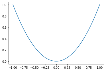
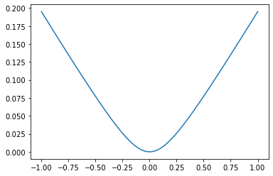
# L2 norm loss is the Euclidean loss function. Advantages: very smmoth near the target and algorithms can use this fact to converge to
# the taraget more slowly, the closer it gets, as follows
l2_y_vals = tf.square(target-x_vals)
x_vals_out = sess.run(x_vals)
l2_y_out = sess.run(l2_y_vals)
plt.plot(x_vals_out, l2_y_out)
[<matplotlib.lines.Line2D at 0x7faa56261af0>]
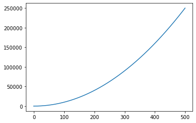
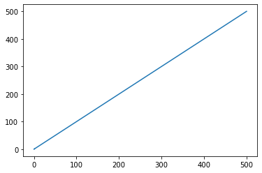
x_vals_1 = tf.linspace(-1., 500., 1000)
target_1 = tf.constant(0.)
l2_y_vals_1 = tf.square(target_1- x_vals_1)
l2_y_out_1 = sess.run(l2_y_vals_1)
plt.plot(sess.run(x_vals_1), l2_y_out_1)
[<matplotlib.lines.Line2D at 0x7faa36a32dc0>]
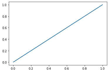
# L1 norm loss is known as the abslute loss function. L1 norm is better for outliners than L2 norm because it is not steep for larger valuse
# One issue to be aware of is that the L1 norm is not smooth at the target and this can result in algorithms not converging well.
l1_y_vals = tf.abs(target-x_vals)
l1_y_out = sess.run(l1_y_vals)
plt.plot(sess.run(l1_y_vals), l1_y_out)
[<matplotlib.lines.Line2D at 0x7faa3676b8b0>]
l1_y_vals_1 = tf.abs(target-x_vals_1)
l1_y_out_1 = sess.run(l1_y_vals_1)
plt.plot(sess.run(l1_y_vals_1), l1_y_out_1)
[<matplotlib.lines.Line2D at 0x7faa368400d0>]
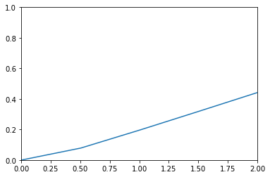
# Pseduo-Huber loss is a continuous and smooth approximation to the Huber loss function. Advantages: L1 and L2
# Examples: delta1 = 0.25 and delta2 = 5
delta1 = tf.constant(0.25)
phuber1_y_vals = tf.multiply(tf.square(delta1), tf.sqrt(1.+ tf.square((target-x_vals)/delta1))-1)
phuber1_y_out = sess.run(phuber1_y_vals)
plt.plot(sess.run(x_vals), phuber1_y_out)
[<matplotlib.lines.Line2D at 0x7faa368febe0>]
phuber1_y_vals_1 = tf.multiply(tf.square(delta1), tf.sqrt(1.+tf.square((target-x_vals_1)/delta1))-1)
phuber1_y_out_1 = sess.run(phuber1_y_vals_1)
x_vals_out_1 = sess.run(x_vals_1)
plt.plot(x_vals_out_1,phuber1_y_out_1)
plt.ylim([0, 1])
plt.xlim([0, 2])
(0.0, 2.0)
delta2 = tf.constant(5.)
phuber2_y_vals = tf.multiply(tf.square(delta2),tf.sqrt(1.+ tf.square((target-x_vals_1)/delta2))-1.)
phuber2_y_out  = sess.run(phuber2_y_vals)
plt.plot(sess.run(x_vals_1), phuber2_y_out)
[<matplotlib.lines.Line2D at 0x7faa3707e430>]

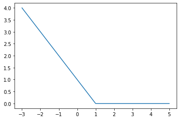
# CLassification loss functions are used to evaluate loss when predicting categorical outcomes.
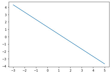
# Hinge loss is mostly used for support vector machines, but can be used in neural networks as well.
x_vals = tf.linspace(-3., 5., 500)
target = tf.constant(1.)
targets = tf.fill([500,],1.)
hinge_y_vals = tf.maximum(0., 1.-tf.multiply(target, x_vals))
hinge_y_out = sess.run(hinge_y_vals)
plt.plot(sess.run(x_vals), hinge_y_out)
[<matplotlib.lines.Line2D at 0x7faa36f8aa30>]
sess.run(targets)
array([1., 1., 1., 1., 1., 1., 1., 1., 1., 1., 1., 1., 1., 1., 1., 1., 1.,
       1., 1., 1., 1., 1., 1., 1., 1., 1., 1., 1., 1., 1., 1., 1., 1., 1.,
       1., 1., 1., 1., 1., 1., 1., 1., 1., 1., 1., 1., 1., 1., 1., 1., 1.,
       1., 1., 1., 1., 1., 1., 1., 1., 1., 1., 1., 1., 1., 1., 1., 1., 1.,
       1., 1., 1., 1., 1., 1., 1., 1., 1., 1., 1., 1., 1., 1., 1., 1., 1.,
       1., 1., 1., 1., 1., 1., 1., 1., 1., 1., 1., 1., 1., 1., 1., 1., 1.,
       1., 1., 1., 1., 1., 1., 1., 1., 1., 1., 1., 1., 1., 1., 1., 1., 1.,
       1., 1., 1., 1., 1., 1., 1., 1., 1., 1., 1., 1., 1., 1., 1., 1., 1.,
       1., 1., 1., 1., 1., 1., 1., 1., 1., 1., 1., 1., 1., 1., 1., 1., 1.,
       1., 1., 1., 1., 1., 1., 1., 1., 1., 1., 1., 1., 1., 1., 1., 1., 1.,
       1., 1., 1., 1., 1., 1., 1., 1., 1., 1., 1., 1., 1., 1., 1., 1., 1.,
       1., 1., 1., 1., 1., 1., 1., 1., 1., 1., 1., 1., 1., 1., 1., 1., 1.,
       1., 1., 1., 1., 1., 1., 1., 1., 1., 1., 1., 1., 1., 1., 1., 1., 1.,
       1., 1., 1., 1., 1., 1., 1., 1., 1., 1., 1., 1., 1., 1., 1., 1., 1.,
       1., 1., 1., 1., 1., 1., 1., 1., 1., 1., 1., 1., 1., 1., 1., 1., 1.,
       1., 1., 1., 1., 1., 1., 1., 1., 1., 1., 1., 1., 1., 1., 1., 1., 1.,
       1., 1., 1., 1., 1., 1., 1., 1., 1., 1., 1., 1., 1., 1., 1., 1., 1.,
       1., 1., 1., 1., 1., 1., 1., 1., 1., 1., 1., 1., 1., 1., 1., 1., 1.,
       1., 1., 1., 1., 1., 1., 1., 1., 1., 1., 1., 1., 1., 1., 1., 1., 1.,
       1., 1., 1., 1., 1., 1., 1., 1., 1., 1., 1., 1., 1., 1., 1., 1., 1.,
       1., 1., 1., 1., 1., 1., 1., 1., 1., 1., 1., 1., 1., 1., 1., 1., 1.,
       1., 1., 1., 1., 1., 1., 1., 1., 1., 1., 1., 1., 1., 1., 1., 1., 1.,
       1., 1., 1., 1., 1., 1., 1., 1., 1., 1., 1., 1., 1., 1., 1., 1., 1.,
       1., 1., 1., 1., 1., 1., 1., 1., 1., 1., 1., 1., 1., 1., 1., 1., 1.,
       1., 1., 1., 1., 1., 1., 1., 1., 1., 1., 1., 1., 1., 1., 1., 1., 1.,
       1., 1., 1., 1., 1., 1., 1., 1., 1., 1., 1., 1., 1., 1., 1., 1., 1.,
       1., 1., 1., 1., 1., 1., 1., 1., 1., 1., 1., 1., 1., 1., 1., 1., 1.,
       1., 1., 1., 1., 1., 1., 1., 1., 1., 1., 1., 1., 1., 1., 1., 1., 1.,
       1., 1., 1., 1., 1., 1., 1., 1., 1., 1., 1., 1., 1., 1., 1., 1., 1.,
       1., 1., 1., 1., 1., 1., 1.], dtype=float32)
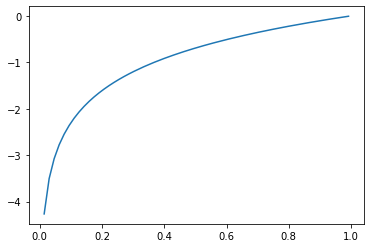
# Cross-Entropy loss for a binary case is also sometimes referred to as the logistic loss function.
xentropy_y_vals = tf.multiply(target, tf.log(x_vals))-tf.multiply((1.-target), tf.log(1.-x_vals))
xentropy_y_out = sess.run(xentropy_y_vals)
plt.plot(sess.run(x_vals), xentropy_y_out)
[<matplotlib.lines.Line2D at 0x7faa369c7940>]
# Sigmoid cross entropy loss is very similar to the previous loss function except we transform the x-values by the sigmoid
# function before we put them in the cross entropy loss, as follows:

xentropy_sigmoid_y_vals = tf.nn.sigmoid_cross_entropy_with_logits(labels=x_vals, logits=targets)
xentropy_sigmoid_y_out = sess.run(xentropy_sigmoid_y_vals)
plt.plot(sess.run(x_vals), xentropy_sigmoid_y_out)
[<matplotlib.lines.Line2D at 0x7faa56580b80>]